Time-Correlated Single Photon Counting (TCPC) is a very sensitive method that allows the measurement of time-resolved fluorescence with a temporal resolution on the order of picoseconds (ps) to nanoseconds (ns). It is a digital technique based on the statistical nature of the quenching of luminescent photons.
The principle of measurement
In TCSPC, the sample under investigation is repeatedly excited by a pulsed light source with a high repetition rate (on the order of kHz and MHz). The moment of emission of the excitation pulse serves as a reference time. During the measurement, the frequency of occurrence of individual photons at different time points from the excitation pulse is recorded. An important condition is that at most one single emitted photon can be detected at each excitation pulse. The excitation pulse represents the START signal for the TCSPC electronics, while the emission signal (registration of the first emission photon) plays the role of the STOP signal. In addition, the fluorescence intensity must be very low in order to register the arrival of single fortons. High internal gain photodetectors are used to detect single photons. In particular, these are photomultiplier tubes (PMTs), microchannel plate photomultipliers (MCP-PMTs) and avalanche photodiodes (APDs).
TCSPC electronics
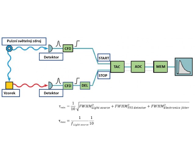
The main components for signal processing using the TCSPC method are a constant fraction discriminator (CFD = Constant fraction discriminator), a time→amplitude voltage converter (TAC = Time-to-Amplitude Converter), an amplifier (between TAC and ADC) and an analog-to-digital converter (ADC = Analogue-to-Digital Converter).
The excitation signal (START) and the signal from the detector (STOP) are fed to the CFD, which produces a logic time signal when the input pulse reaches some given fraction of its amplitude. The time→amplitude converter starts to generate a voltage linearly increasing with time due to the time START signal. This voltage stops being generated when the converter detects the arrival of the time STOP signal. The TAC output voltage signal is then proportional to the time interval between the START and STOP signals. This voltage is further processed by the A/D converter (ADC) and stored in the computer memory. For a large number of START-STOP cycles, the measured histogram then corresponds to the fluorescence quenching process.
Direct vs. reverse mode of operation
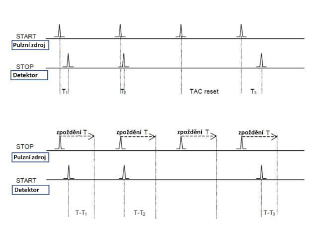
When using pulse sources with a high repetition rate, the direct mode measurement described above has a clear disadvantage. The vast majority of START-STOP cycles are indeed triggered by the START signal, but the STOP signal does not arrive before the next START pulse starts and the TAC is therefore constantly in reset mode. For this reason, the TCSPC electronics are often configured to operate in the so-called reverse mode. The difference is that the emission signal is used as a START signal for the voltage rise on the TAC and the excitation pulse is used as a STOP signal. The reference pulses from the light source are delayed to make them arrive at the TAC later than the START signal.
Time resolution
The TCSPC method can measure fluorescence lifetimes ranging from ~5 ps to ~50 us. The lower limit τmin (achievable temporal resolution) is related to a quantity called the Instrument Response Function (IRF). An ideal system with extremely narrow excitation pulse widths, an infinitely accurate detector and TCSPC electronics having zero jitter corresponds to an IRF in the form of an infinitesimal curve (d-function). Deviation from these ideal conditions leads to a broadening of the instrument response function. The most common limiting factors for the achievable temporal resolution are the temporal width of the excitation pulses and the detector's ability to determine the exact time of arrival of each photon. The measured fluorescence quenching kinetics is the result of the convolution of the IRF with the actual time response. Therefore, in the case of a fast fluorescence response, additional mathematical processing (deconvolution) of the measured decay curve is required. Numerical deconvolution allows to resolve lifetimes corresponding to approximately 10% of the half-width (FWHM) of the instrument response function (see the factor of 1/10 in the expression for τmin at the bottom of the illustration). A sample that scatters light strongly (scattering occurs several orders of magnitude faster than fluorescence and can thus be considered with a good approximation as τ→0) is most often used for experimental IRF determination.
The upper limit τmax is determined by the repetition rate of the pulsed excitation source and the dark count rate of the detector. If the fluorescence signal does not decay before the next pulse hits the sample, a stationary background is created, thus limiting the dynamic range. If the fluorescence signal has time to fall to 1/10,000 of its peak value between two consecutive excitation pulses, then the longest measurable lifetime is estimated as 1/10 of the excitation source period (see expression for τmax at the bottom of the illustration). To avoid a significant decrease in measurement accuracy, the maximum value of the number of dark detections should numerically correspond to 5% of the value of the repetition rate of the excitation source (i.e., for example, a detector with 50000 cps should be used in combination with a light source with a frequency > 1 MHz).